 Spectral Analysis of Earth Samples using Factor Analysis
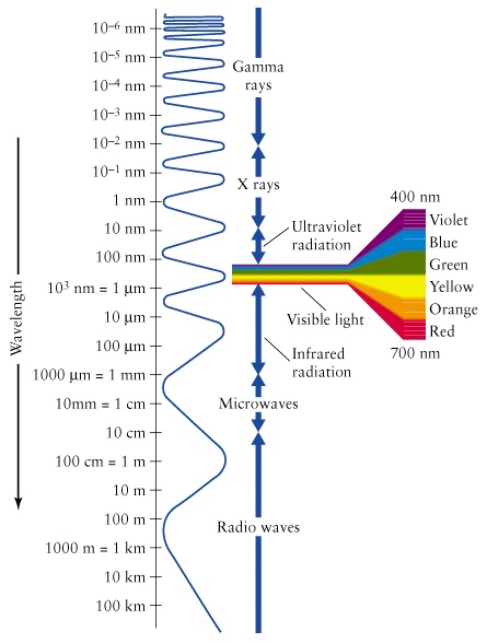
Marine geologists and physicists have used colour, which is the human eye’s perception of reflected radiation in the visible region of the electromagnetic spectrum to describe marine sediment cores for many years. Sediment colour is usually determined visually by comparison to colour charts. Such colour-chart analysis is qualitative and inexact because no two observers have the same colour perception. Colour also tends to obscure differences in visible spectra because similar colours may result from the mixing of different spectral wavelengths, a condition termed metamerism. Many of the problems related to qualitative colour analysis can be overcome by using diffuse-reflectance spectrophotometry and a suitable technique for analyzing the data.
 In a previous Ocean Drilling Program conducted by Texas A&M University, they measured and analyzed near-ultraviolet/visible/near-infrared spectral data from core samples recovered from Ocean Drilling Program. In their work, they used the software SysStat (version 7.0.1), a product of SPSS Inc to factor analyze the data and generated plots of factor scores to determine trends in temporal changes. The primary method used to interpret factors in this study is factor description diagrams, which are plots of the importance of each wavelength through the wavelength range analyzed.
In this experiment, we will do Factor Analysis by the Principal Components Method and compare the resulting factor description curve with the previous results. Spectral Data obtained in previous research by John E. Damuth and William L. Balsam was compared with the arrived results. The factors curves obtained from the previous research had been compared with the factor curves obtained in the proposed experiment.
Sample of Reflectance Spectra Data Data
The following is the one sample of such records from the Ocean Drilling Program. These spectrographic data were provided by Texas A&M University and are freely available on the internet for this kind of research. The first three values are used to identify the sample. They are Core- section, interval (cm) and Depth (mbsf-meters below sea-floor). And the remaining 61 numbers are the measure of Spectral values (per cent reflectance). But, for the proposed analysis, the whole data set of 1290 records will be used.
Core-section, interval (cm) Depth (mbsf) [250 nm 260 nm 270 nm ………… 850 nm – 61 Values]
1X-1,7-8 0.07 8.1 8.26 8.9 9.94 11.36 13.03 14.73 16.69 19.04 20.33 20.78 21.64 22.67 24.54 26.16 27.63 29.17 30.99 32.53 33.79 35.09 35.83 36.38 36.91 37.63 38.52 39.53 40.52 41.44 42.32 43.18 43.86 44.39 44.77 45.06 45.28 45.43 45.56 45.66 45.77 45.87 45.99 46.1 46.18 46.24 46.29 46.42 46.54 46.64 46.84 47.03 47.29 47.59 47.76 48.06 48.3 48.55 48.75 49.01 48.88 49.0
The Diagram Explaining the Steps in Analysis
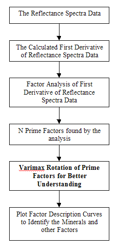
Steps in Proposed Analysis
Implementation Results and Discussion
 The primary method used to interpret factors in this study is factor description diagrams, which are plots of the importance of each wavelength (i.e., factor loading) through the wavelength range analyzed (factor pattern curve). The resulting factor description curve is then compared to first-derivative curves for known minerals, combinations of minerals and sediment components. Balsam and Deaton (1991) demonstrated that this method can be used to identify iron oxide and clay mineral factors in modern Atlantic Ocean sediments. For Sites 1165 and 1167, all the factor description curves can be related to first-derivative curves for known minerals or sediment components.
An example of the interpretation of a factor description curve by comparison to the first-derivative from a known sample containing hematite and goethite (from Balsam et al., 1997). Squares = first derivative values, circles = factor loading.
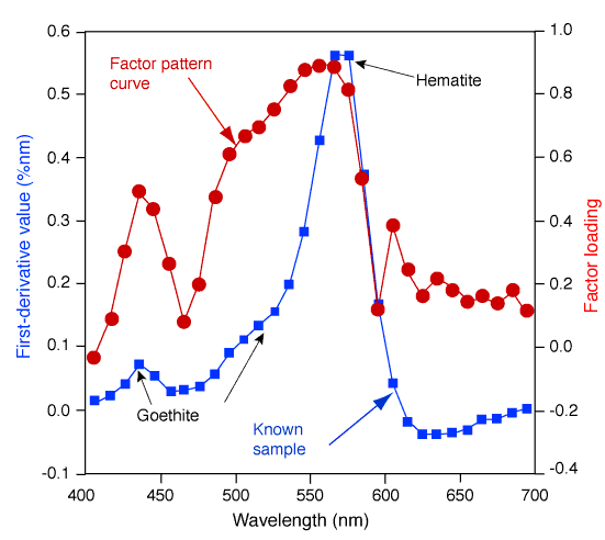
Example of interpretation of a factor description curve
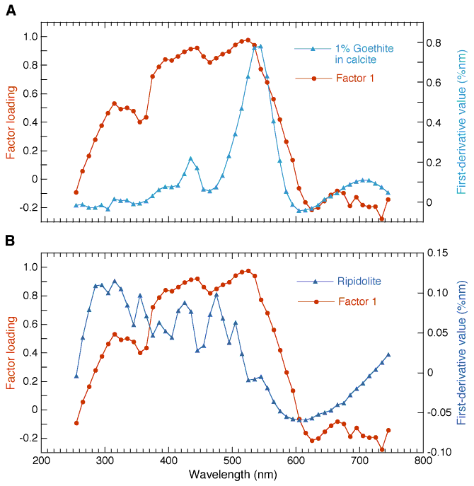
Factor 1
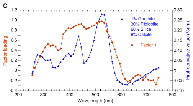
Factor 1 is interpreted as representing a combination of minerals including goethite and chlorite, most likely ripidolite. A, B. This interpretation is based on the comparison of the first derivative peaks derived from spectral analysis of standards to peaks in the factor loading curve. The standard goethite is Hoover Color Corporation Synox HYG10, yellow, and is a manufactured sample. Ripidolite, one of our natural chlorite standards, is sample CGA-2 from the Clay Minerals Repository and is from Flagstaff Hill, California. C. This curve clearly demonstrates the spectral dominance of goethite, even at low concentrations, and how the intermixing of two minerals may affect their combined spectrum. The silica and calcite in the known mineral mixture shown are white and do not influence the spectrum in the wavelength range we analyzed
Interpretation of a factor description curve of Factor 1
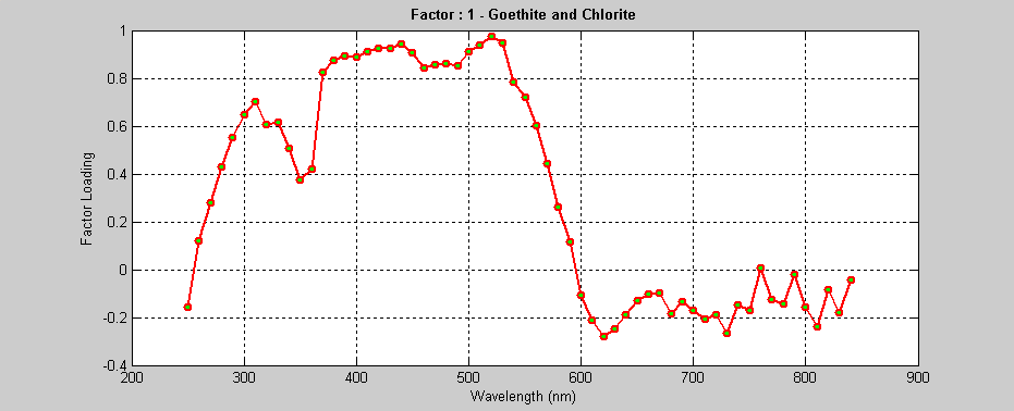
Factor 1 Curve Obtained in this Experiment
Factor 2
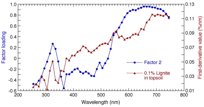
Factor 2 is interpreted as an organic matter factor. This interpretation is based on the comparison of the factor loading curve for Factor 2 to the spectral curve of a small amount of lignite (0.1%) mixed with commercial topsoil. Note: We do not mean to imply that ocean-floor sediments contain material similar to topsoil, rather we use this mixture because we imply that this factor contains both mature, refractory organic matter and immature, young organic matter such as that found in topsoil.
 Interpretation of a factor description curve of Factor 1
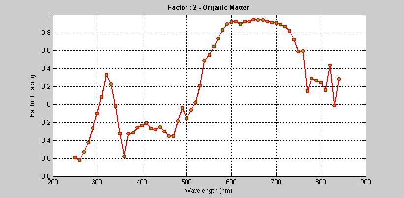
Factor 2 Curve Obtained in this Experiment
Factor 3
Factor 3 is interpreted as being influenced by both illite and montmorillonite. Comparison of the factor loading curve for Factor 3 to spectral patterns for (A) montmorillonite and (B) illite demonstrates that the factor loading curve shares first derivative peaks with both of these clay minerals. Our montmorillonite sample is API 25 from Upton, Wyoming, and is described as 100% montmorillonite (bentonite). The illite sample is API 35 (Wards 46E-4100) from Fifthian, Illinois, and is described as 100% illite.
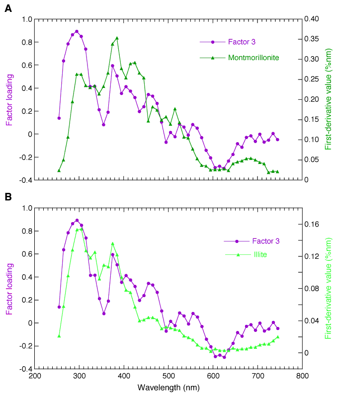
Interpretation of a factor description curve of Factor 3
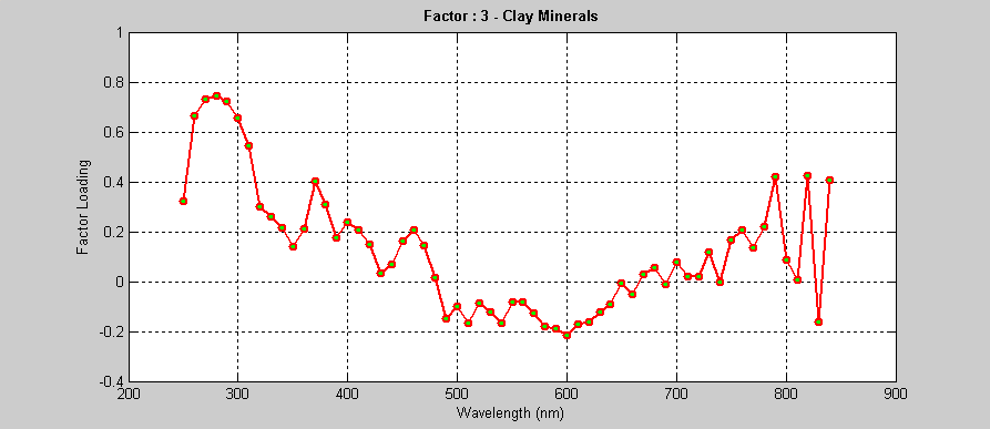
Factor 3 Curve Obtained in this Research
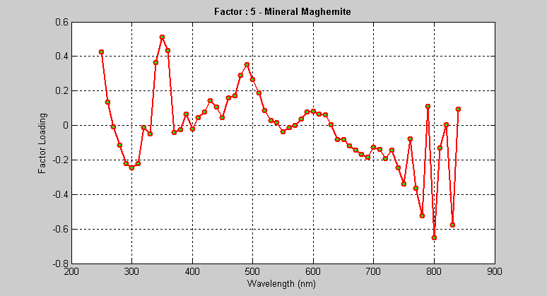
Factor 4
Factor 4 is interpreted as containing maghemite and some other undetermined mineral. The comparison of our factor loading curve to the first derivative curve for a standard sample of maghemite displays several peaks in common. However, the 495-nm factor loading peak is not present in our standard and the maghemite first-derivative peak at 665 nm is not present on the factor loading curve; this suggests the presence of at least one additional mineral influencing the factor. Our maghemite standard is manufactured by Pfizer (their number 2230).
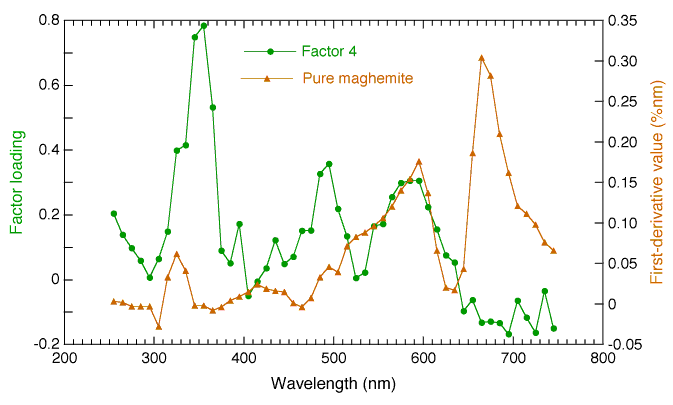
Interpretation of a factor description curve of Factor 4
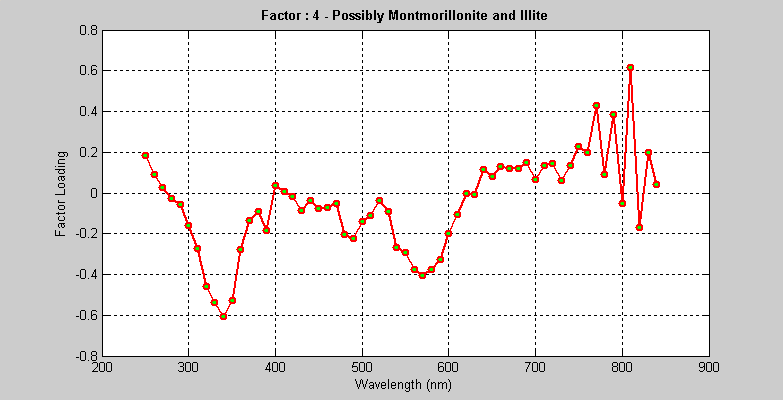
Factor 4 Curve Obtained in this experiment
Factor 5
Factor 5 is interpreted as representing primarily hematite plus an unidentified mineral. The comparison of the factor loading curve to the first derivative curve for 1% hematite in calcite clearly indicates the presence of hematite. However, the large factor loading peak at 335 nm and the smaller peaks centred at 400 nm indicate the presence of another mineral, probably a clay mineral, that has peaks in the NUV and shorter wavelengths of the VIS (for example see the curves for ripidolite, illite, and montmorillonite in previous figures).
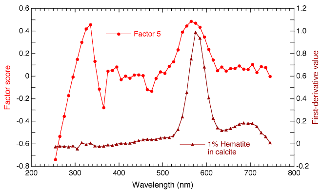
Interpretation of a factor description curve of Factor 5
Factor 5 Curve Obtained in this Research
Summary
Generally, comparing the spectra of invisible as well as visible regions is very hard for the naked eye since the human eye is not a very accurate tool to process the colour information available in spectra. But using the factor curves of this research, one can easily compare the spectra from either invisible or visible regions.
By using these factor curves, we can predict the presence of a particular element or mineral or sediment in the sample under investigation. Since the spectra of specimens were from oceanographic research, the prepared factor curves can be used for any other future research related to oceanography and other fields of science.
 Take Me to Afarion ns-3 iPlayground