Based on my experience and interactions with lots of intelligent scholars from different parts of the world, I can definitely say that a Quality Table of results and a good set of analytical Graphs are more important for publishing a paper in a reputed journal and submitting a thesis to a reputed university.
Of course, we may have a genuine concept or innovation for our research submission – but proving its goodness by comparing its performance with other similar methods is an important aspect in every research publication.
While doing research on any kind of algorithms and models related to networks using a simulator such as ns-2, ns-3, and OmNet++, proving the good working of a proposed algorithm or model with suitable metrics is an important aspect needed for publishing that research.
My previous articles [1] and [2] explained the way of creating simple analytical results :
Trace Analysis of TCP Flows Under ns-3 MANET/ FANET/ VANET/ WSN Scenario
But, managing a scholarly research submission of a journal paper or thesis will not be possible with this kind of elementary analysis.
This article explains the professional way of generating Quality Tables and graphs for a journal paper and a Ph.D thesis report from a batch of simulations.
Batch Simulations
You can not generate quality graphs and tables with a single run of a typical network simulation. Often, undergraduate students will do their analysis based on a single run of a network simulation. But, for a scholarly research submission, one will need statistically significant and more comparable results that can not be generated from a single run of a network simulation. So, for that, we need to run one simulation script with different parameters and for several iterations or repetitions of one simulation with different random “seed”.
As a simple example, if we need to evaluate the performance of 5 different routing protocols under 6 different network densities under ns-2, then we may need to run the same simulation for 5×6 times (30 times). However, it will not be sufficient; we have to simulate different node orientations on the 6 different network densities. So for each network density, we need to test 10 different network topologies (with 10 different, random node orientations – it means, 10 iterations or repetitions). So, in this simple example, we need to run one simulation for 5x6x10 times (300 times) and only take the average of 10 iterations to prepare the final tables and graphs.
Not only that. While running the simulation for 300 times, we have to generate and log the trace output files with suitable names. For example, if a simulation generates one event trace output and another custom trace output, then for each run of the simulation, it should generate two trace output files with distinct file names. So at the end of the batch simulation run, our hard disk will end up with 600 trace files with distinct file names – and after consuming several hours of “run time”, it may eaten-up several GB’s of disk space.
But a typical scholarly research-level submission will need a batch simulation and analysis that is even much more complex than the above simple example.
We can not manually run the simulation by hand 300 times with different parameters – it will be a tedious process and will lead to human errors (generally, typographical errors on numeric values). So we need to automate this by writing a shell script to make that one network simulation script run 300 times and generate 600 trace output files with distinct file names.
Shell Script to Do “Batch Simulation Runs”
The following is a pseudocode of a typical shell script that can be used for doing batch runs of a simulation.
Caution: Here, it is intentionally presented as a pseudo-shell-script – so you can not run it on any shells of Linux. One should learn UNIX shell scripting language and properly write their own “BatchRun.sh”
# BatchRun.sh
# Caution: it is only a pseudo-shell-script.
RoutingProtocols = { AODV, DSDV, DSR, MyAODV, MyDSR}
NetworkDensities= {50, 100, 150, 200, 250, 300}
for iteration = 1 to 10
begin
for routing in RoutingProtocols
begin
for density in NetworkDensities
begin
TraceFileName1= string(iteration + routing + density ) + “.tracefile1.tr”
TraceFileName2= string(iteration + routing + density ) + “.tracefile2.tr
ns NetworkSimulation.tcl iteration routing density TraceFileName1 TraceFileName2
// for old ns-3 : waf –run NetworkSimulation iteration routing density TraceFileName1 TraceFileName2
// for new ns-3-dev : ns3 –run NetworkSimulation iteration routing density TraceFileName1 TraceFileName2
end
end
end
A Typical BatchRun.sh
Note: While passing parameters to a simulation script, then the simulation script should process those passed parameters and act accordingly.
Analysis of Batch Simulation Outputs
We have to extract the output parameters such as PDF, e2e delay, througput etc., from the previously stored 600 trace output files.
For that, we may need to write some custom ‘Awk” scripts for doing trace analysis to prepare graphs or charts like:
- Number of Nodes Vs PDF
- Number of Nodes Vs Throughput
- Number of Nodes Vs Delay
- Number of Nodes Vs MAC Load
- Number of Nodes Vs Network Load
- Number of Nodes Vs Routing Load
- Number of Nodes Vs Average Consumed Energy
- Number of Nodes Vs Average E2E Delay
- etc., etc.,
The following shell scripts will do the trace analysis on the 600 trace files that were generated during the batch simulation runs.
It is a batch-trace-analysis script – it will iteratively do trace analysis on the 600 trace files using suitable “awk” script files and will store the average results of the 10 iterations/repetitions in output files with distinct names.
Plotting the Outputs
For plotting the outputs of trace analysis, one may use xgraph, GnuPlot, or Matplotlib etc.,. You can see a lot of graph plotting options at [5] and [6].
Here, I present a way of using GnuPlot to create elegant graphs from the previous trace analysis outputs of batch-trace-analysis.
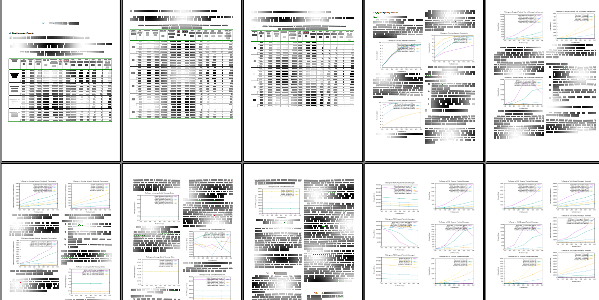
Typical output from a batch simulation and Analysis.
The following is the results section of a rough draft of a typical paper prepared for a journal publication. Here we are using the tables and graphs that were generated by the automated batch-simulation-run script, batch-trace-analysis script and the graph-plotting script. So, if we write these scripts correctly, then these scripts will run the simulation in an automated way and will create elegant graphs in an effortless way.
Conclusion
The way of doing batch-simulation-run and batch-trace-analysis on ns-2, ns-3 and OmNet++ may differ a little bit with respect to the simulator. Particularly, ns-3 and OmNet++ will log trace outputs in a different way. So one should design these scripts as per the simulator of their choice.
References
- https://www.projectguideline.com/an-elementary-research-on-uwsn-using-ns-2/
- https://www.projectguideline.com/trace-analysis-of-tcp-flows-under-ns-3-manet-fanet-vanet-wsn-scenario/
- http://nile.wpi.edu/NS/analysis.html
- http://intronetworks.cs.luc.edu/current1/uhtml/ns2.html
- https://www.ubuntupit.com/best-plotting-tools-for-linux-for-creating-scientific-graphs/
- https://www.toptal.com/designers/data-visualization/data-visualization-tools
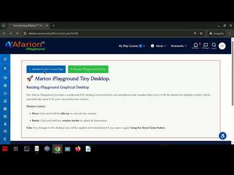
 Take Me to Afarion ns-3 iPlayground