#Post Title

Introduction.

Even after a lot of theoretical understanding of particular networking technology, for a beginner, understanding the way in which they are implemented in a practical system or in a simulator will be a challenging task.

While interacting with the scholars and students, I often realized that most of them are doing their projects or research on underwater communication systems without really understanding the very physical nature of different types of underwater communication technologies. Even I saw some of them try to use a MANET routing protocol or MANET MAC protocol to simulate an acoustic underwater network. This article is for such beginners to make them do a simple UWSN simulation project in a genuine way.

Software Needed for UWSN under ns-2

A genuine routing protocol evaluation project can be implemented using Aquasim underwater network extension of ns-2. Even we can do serious research work on some other aspects of UWSN also using this extension( like in MAC layer, transport layer etc.,)

You can find the procedure for installing Aquasim at the following link:

Installing Aqua-Sim in Ubuntu 16.04 LTS – Underwater Sensor Network Simulation with ns-2

The simulated UWSN can be visualized in 3D using Aqua-3D tool. Aqua-3D is nothing but an enhanced version of NAM. NAM can only be used to visualize a network in 2D. But Aqua-3D can be used to visualize the simulated UWSN in 3D.

The procedure for installing Aqua-3D can be found at the following link:

Installing Aqua-3D Visualization Tool In Ubuntu 16.04 LTS and Visualizing Aqua-Sim Underwater Network Simulations

Planing a Generic Simulation Script

To to a genuine evaluation on different routing protocols, we have to use common parameters in all the cases of routing algorithms. I mean, except for the name of the routing protocol, we should not change any other node configuration or network configuration parameters in the simulation. I mean, the performance of the protocols should be evaluated under common network conditions. Some students and scholars may use separate simulation scripts with different settings during their evaluation – it is not the genuine way of doing scholarly research work- it will lead to un-comparable, wrong, “cooked-up” results.

For example, if we write a simulation script for evaluating the performance of the three underwater routing protocols (1) UWFlooding, (2) VBF and (3) DBR, then the same script should be used to evaluate all the three UWSN routing protocols. For that, we have to configure some additional parameters according to that routing protocol (using a switch or if conditions).

In the generic simulation script that we write for evaluating three routing protocols, only an extra setting for width parameters will be needed for VBF. For other cases UFFlooding and DBR, the width parameter is not necessary. So this situation can be handled easily with a simple ‘if condition check’ in that common script – all other parameters should be kept in common during the three repeated runs of the simulation script for three routing protocols – then only the evaluation will be genuine.

The script may contain additional code for handling files to store the event trace outputs, nam trace outputs and custom data outputs. The name of those files should be created dynamically with respect to the name of the selected protocol (which is passed through the command line). One such script can be easily made using the existing example script which is readily available with Aquasim installation.

Running the Simulation Script

In this case, that command line parameter may be UWFlooding or Vectorbasedforward or DBR. So if your simulation script is in the name “SimpleUWSN.tcl”, then you should run it as follows :

$ns SimpleUWSN.tcl UWFlooding.

Now the simulation script will run a UWSN with UWFlooding routing protocol and store the trace outputs in a file which was created dynamically with the name in it (like “TheOutput-UWFlooding.tr” or “TheOutput-UWFlooding.nam” etc.,). In addition to that we will see some outputs in the terminal that were logged by the aquasim extension itself.

$ns SimpleUWSN.tcl Vectorasbedforward.

So, now the simulation script will run a UWSN with Vectorbasedforward routing protocol and store the trace outputs in a file which was created dynamically with the name in it (like “TheOutput-Vectorasbedforward.tr” or “TheOutput-Vectorasbedforward.nam” etc.,)

$ns SimpleUWSN.tcl DBR.

Now the simulation script will run a UWSN with DBR routing protocol and store the trace outputs in a file which was created dynamically with the name in it (like “TheOutput-DBR.tr” or “TheOutput-DBR.nam” etc.,)

Instead of running it manually, we may automate it using a shell script. For research-level simulations, we may need to run a batch of simulations – in that case, a shell script based automation of running the simulation with different parameters is good practice.

The Numerical Outputs of our Simulation Runs

An Elementary Analysis with some Elementary Graphs For Better Understanding of the Result

For the comparison purpose, we can prepare some elementary graphs using the above numerical values.

Comparison of Total Sent Packets with the Three Routing Algorithms.

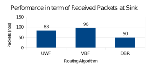
In the above graph, VBF performed well in terms of total sent packets.

Comparison of Cumulative Delays Achieved by the Three Routing Algorithms.

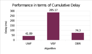
As shown in the above graphs, UWF(Underwater Flooding) performed well in terms of total sent packets.

Comparison of Total Consumed Energy of the Network with the Three Routing Algorithms.

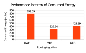
As per the above graphs, VBF performed well in terms of total Battery Energy Consumption.

So as the result of this elementary analysis, we can say that VBF performed better than other two compared routing protocols. But keep in mind that, these are the result of a single simulation run (one run with each routing protocol). For confirming these results one should repeat each simulation several times (even with different node configurations and a different number of nodes) and should take an average of results of each batch of runs. Then only we will get more significant, distinguishable and comparable results.

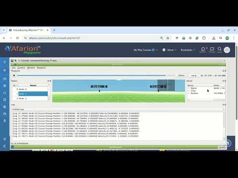
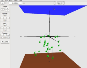
Some 3D Output of Aqua-3D

The following figure shows an example of the 25 Node Underwater Network scenario which is Visualized with Aqua3D. The brown square at the bottom is representing the underwater ground. The blue square at the top is representing the sky. The middle node is at the water surface. The Aqua3D can visualize packet transmissions as expanding spheres and even can visualize packet drop events also.

Additionally, one may try the following analysis/graphs:

By using the “custom logged” trace files, and the default event trace file of ns-2, we can prepare more results. For that, we may need to write some custom ‘Awk” scripts for doing trace analysis.

Number of Nodes Vs PDF
Number of Nodes Vs Throughput
Number of Nodes Vs Delay
Number of Nodes Vs MAC Load
Number of Nodes Vs Network Load
Number of Nodes Vs Routing Load
Number of Nodes Vs Average Consumed Energy
Number of Nodes Vs Average E2E Delay
etc., etc.,

Summary

In this article, as proof of concept, we explained the way of doing a genuine evaluation of UWSN routing protocols under ns-3.

But, for producing quality output for journals and doing a scholarly thesis, these kinds of simple results based on a ‘single run’ evaluation will not be sufficient. For producing quality outputs we have to repeat the simulations several times with different random seeds and take the average of the results of each batch of runs.

For example, if we need to do a “Network Density vs Performance” analysis, we may need to run the simulation with different numbers of nodes and repeat the simulation with the three routing protocols. These three sets of runs should be repeated for N times (N iterations with different random seeds) and take the average of that N iterations. Now only we will end up with meaningful graphs.

For doing such scholarly experiments and evaluation, we have to write several awk scripts for doing trace analysis and have to write some shell scripts to automate these batch runs of simulations and analysis. This article does not address those aspects of batch simulations and analysis.
Please note that, while doing scholarly research work all the numerical results, tables and graphs should be automatically generated while running a “Trace Analysis” shell script. That king of automated generation of results will give more reliability and trustability to the people who are going to validate or judge your work.