Caution :

If you try to use Directed Diffusion routing under a highly-mobile condition, then the performance of the Directed Diffusion routing will become very worst. Some of the papers that you see in literature may try to hide this fact.

Further, this evaluation is an elementary evaluation which considered only “time vs performance” as a metric. So any serious research on this routing protocol will need a lot of iterative simulations and more advanced analysis.

Introduction

Directed Diffusion is a data-centric routing algorithm for sensor networks. Its key features are named attribute-value pairs and path reinforcement. Directed diffusion is a reactive routing protocol which creates paths based on need, not ahead of time. Sensed data is stored in attribute-value pairs. When a node known as a sink node wants information about a particular attribute, it broadcasts interest messages to its neighbors. These interest messages are flooding through the network and are added to each node’s interest cache. Each interest record in this cache has one or more gradients which correspond to neighbor nodes that transmitted the interest. The gradient also stores the rate at which data is desired, the duration of the interest, and a timestamp. When a node generates data that matches an interest in its cache, it sends the data back to the source along the gradients. Intuitively, the data is drawn to the sink through the gradients. The sink node may reinforce the shortest path (i.e., the one with the fastest response) by sending an interest with a higher data rate along that path. Intermediate nodes propagate the reinforcement by examining a local cache of recently sent data messages. The data cache also prevents loops in data delivery. Slower data paths may be sent negative reinforcement, i.e. interest messages with a slow data rate to save network bandwidth. If a sink wants to continue receiving data it must periodically reinforce the path to update the timestamp and duration in the gradients.

Consider a simple sensor network for remote surveillance of a region. In practice, such a network might consist of several hundreds or thousands of sensor nodes deployed within that region. In some cases, the sensor field may be deployed in a regular fashion (e.g. a 2-dimensional lattice, or a linear array) within that region. More generally, however, communication and networking protocols cannot assume structured sensor fields.

The human operator’s query would be transformed into an interest that is diffused towards nodes in regions X or Y. When a node in that region receives an interest, it activates its sensors which begin collecting information about pedestrians. When the sensors report the presence of pedestrians, this information returns along the reverse path of interest propagation. An important feature of directed diffusion is that interest and data propagation and aggregation are determined by localized interactions.

Features of Directed Diffusion 

 Data Centric, Attribute-Value pairs
 Events Flow towards the originator across multiple paths
 Interest and task Propagation initiated at the sink and propagated through flooding
 Initial gradient setup by node, where gradient consists of data rate value and direction
 Data delivery along reinforced path, selected as an empirically low delay path
 Experimentation required for choosing local rule to use for negative reinforcement
 Average energy dissipation of directed diffusion is better than flooding and omniscient multicast (shortest-path from source to sink)
 Average delay of directed diffusion is almost the same as omniscient multicast but much less than flooding

Disadvantages of Directed Diffusion

 Congestion recovery mechanism Unavailable
 Congestion performance of protocol not verified
 Power efficiency of MAC Layer undefined
 Experiments needed to find the best negative-reinforcement rule (power efficient)

The Main Aspects of Directed Diffusion

Interest Propagation

 

     
Flooding will be used for interest propagation. Constrained or Directional flooding an also be used based on location. Directional Propagation may be used based on previously cached data.

Data Propagation

 

 Data Propagation is Reinforcement to single path delivery.
 Data Propagation can be Multipath delivery with probabilistic forwarding.
 Data Propagation cam be Multipath delivery with selective quality along different paths

Reinforcement

 

The Reinforcement process Reinforce one of the neighbor after receiving initial data. It will be based on the following factors
 Neighbor(s) from whom new events received.
 Neighbor who’s consistently performing better than others.
 Neighbor from whom most events received.

Negative Reinforcement

The Negative Reinforcement Explicitly degrade the path by re-sending interest with lower data rate and improve the quality of data transfer in Reinforced Paths.

 

 

Steps in Directed Diffusion 

Interests and Gradients

In directed diffusion, task descriptions are named by, for example, a list of attribute-value pairs that describe a task. It is called as interest.

type = four-legged animal // detect animal location
interval = 20 ms // send back events every 20 ms
duration = 10 seconds // for the next 10 seconds
rect = -100, 100, 200, 400 // from sensors within rectangle

 an interest is injected into the network at some (possibly arbitrary) node in the network (sink)
 suppose a task, with a specified type and rect, a duration of 10 minutes and an interval of 10ms
 the interval parameter specifies an event data rate for each active task, the sink periodically broadcasts an
 interest message to each of its neighbors
 the initial interest contains a larger interval attribute
 interest is periodically refreshed by the sink
 the refresh rate is a protocol design parameter that trades off overhead for increased robustness to lost interests
 every node maintains an interest cache
 two interests are distinct, if their type attribute differs, their interval attribute differs, or their rect attributes are (possibly partially) disjoint
 interest entries in the cache do not contain information about the sink
 The definition of distinct interests also allows interest aggregation
 this initial interest may be thought of as exploratory
 an entry in the interest cache has several fields
 a timestamp field indicates the timestamp of the last received matching interest
 the interest entry also contains several gradient fields, up to one per neighbor
 the direction of the gradient will point the node from which the interest was received and the direction to which the data should be forwarded.
 each gradient contains a data rate field requested by the specified neighbor and a duration field
 when a node receives an interest, it checks to see if the interest exists in the cache
 if no matching entry exists, the node creates an interest entry
 this entry has a single gradient towards the neighbor from which the interest was received
 individual neighbors, so any locally unique neighbor identifier may be used (802.11 MAC or Bluetoothcluster addresses)
 if there exists an interest entry, but no gradient for the sender of the interest, the node adds a gradient with the specified value
 it also updates the entry’s timestamp and duration fields appropriately
 if there exists both the node simply updates the timestamp and duration fields
 when a gradient expires, it is removed from its interest entry
 when all gradients for an interest entry have expired, the interest entry itself is removed from a cache
 after receiving an interest, a node may decide to re-send the interest to some subset of its neighbors
 to its neighbors, this interest appears to originate from the sending node
 interests diffuse throughout the network
 there are several possible choices for neighbors
 simplest is to rebroadcast the interest to all neighbors
 in the absence of information about which sensor nodes are likely to be able to satisfy the interest, this is the only choice
 when a node receives an interest from its neighbor, it has no way of knowing whether that interest was in response to one it sent out earlier, or is an identical interest from another sink an the “other side” of that neighbor
 such two-way gradients can cause a node to receive one copy of low data rate events from each of its neighbors
 this technique can enable fast recovery from failed paths or reinforcement of empirically better paths, and does not incur persistent loops
 a gradient specifies both a data rate and a direction in which to send events (value and direction)
 the directed diffusion paradigm gives the designer the freedom to attach different semantics to gradient values
 gradient values might be used to probabilistically forward data along different paths, achieving some measure of load balancing
 interest propagation sets up state in the network to facilitate “pulling down” data towards the sink
 the interest propagation rules are local
 a sensor network may support many different task types
 interest propagation rules may be different for different task types
 some elements of interest propagation are similar: the form of the cache entries, the interest re-distribution rules etc..
 we hope to cull these similarities into a diffusion substrate at each node, so that sensor network designers can use a library of interest propagation techniques for different task types

 Data Propagation

 sensor node that’s in specified rect processes interests
 node tasks its local sensors to begin collecting samples
 algorithms simply match sampled waveforms against a library of presampled, stored waveforms
 the algorithms usually associate a degree of confidence with the match
 a sensor node that detects a target searches its interest cache for a matching interest entry
 when it finds one, it computes the highest requested event rate among all its outgoing gradients
 the node tasks its sensor subsystem to generate event samples at this highest data rate
 in our example, this data rate is initially 1 event per second
 the source then sends to each neighbor for whom it has a gradient, an event description every second of the form:

Thus, for example, a sensor that detects an animal might generate the following data.

type = four-legged animal // type of animal seen
instance = elephant // instance of this type
location = 125, 220 // node location
intensity = 0.6 // signal amplitude measure
confidence = 0.85 // confidence in the match
timestamp = 01:20:40 // event generation time

 this data message is, unicast individually to the relevant neighbors
 a node that receives a data message from its neighbors attempts to find a matching interest entry in its cache
 if no match exists, the data message is silently dropped
 if a match exists, the node checks the data cache associated with the matching interest entry
 this cache keeps track of recently seen data items
 it has several potential uses, one of which is loop prevention
 if a received data message has a matching data cache entry, the data message is silently dropped
 the received message is added to the data cache and the data message is resent to the node’s neighbors
 by examining its data cache, a node can determine the data rate of received events
 to resend a received data message, a node needs to examine the matching interest entry’s gradient list
 if all gradients have a data rate that is greater than or equal to the rate of incoming events, the node may simply send the received data message to the appropriate neighbors
 if some gradients have a lower data rate than others, then the node may downconvert to the appropriate gradient
 a node that has been receiving data at 100 events per second, but one of its gradients is at 50 events per second
 the node may only transmit every alternate event towards the corresponding neighbor
 it might interpolate two successive events in an application-specific way
 loop prevention and downconversion illustrate the power of embedding application semantics in all nodes
 this design is not pertinent to traditional networks, it is feasible with application-specific sensor networks
 it can significantly improve network performance

Reinforcement

 in the scheme we have described so far, the sink initially diffuses an interest for a low event-rate notification (1event per second)
 once sources detect a matching target (send low-rate events)
 after the sink starts receiving these low data rate events, it reinforces one particular neighbor in order to “draw down” higher quality (higher data rate) events
 one example of such a rule is to reinforce any neighbor from which a node receives a previously unseen event
 to reinforce this neighbor, the sink resends the original interest message but with a smaller interval (higher data rate).
 when the neighboring node receives this interest, it notices that it already has a gradient towards this neighbor and that the sender’s interest specifies a higher data rate than before
 if this new data rate is also higher than existing gradient, the node must also reinforce at least one neighbor
 how does it do this?
 the node uses its data cache for this purpose (again local rule choices)
 this node might choose that neighbor from whom it first received the latest event matching the interest
 through this sequence of local interactions, a path is established from source to sink transmission for high data rate events
 the local rule we described above, then, selects an empirically low delay path
 it is very reactive to changes in path quality
 one path delivers an event faster than others, the sink attempts to use this path to draw down high quality data
 because it is triggered by receiving one new event, this could be wasteful of resources
 these choices trade off reactivity for increased stability
 exploring this tradeoff requires significant experimentation and is the subject of future work
 the algorithm described above can result in more than one path being reinforced
 e.g.: if the sink reinforces neighbor A, but then receives a new event from neighbor B, it will reinforce the path through B
 one mechanism for negative reinforcement is to time out all high data rate gradients in the network unless they are explicitly reinforced
 another approach is to explicitly degrade the path through A by resending the interest with the lower data rate
 when A receives this interest, it degrades its gradient towards the sink
 if all its gradients are now low data rate a negatively reinforces those neighbors that have been sending data to it at a high data rate
 this sequence of local interactions ensures that the path through A is degraded rapidly, but at the tost of increased resource utilization
 we need to specify what local rule a node uses in order to decide whether to negatively reinforce a neighbor or not
 this rule is orthogonal to the choice of mechanism for negative reinforcement
 one plausible choice for such a rule is to negatively reinforce that neighbor from which no new events have been received within a window of N events or time T
 such a rule is a bit conservative and energy inefficient
 significant experimentation is required before deciding which local rule achieves an energy efficient global behavior
 internodes on a previously reinforced path can apply the reinforcement rules
 useful to enable local repair of failed or degraded paths
 our description so far has glossed over the fact that a straightforward application of reinforcement rules will cause all nodes downstream of the lossy link to also initiate reinforcement procedures
 this will eventually lead to the discovery of one empirically good path, but may result in wasted resources

A Typical interest issued from Sink

What sharp temperature variations (delta T > 10 degrees in the course of 1 minute) have been observed in the southeast quadrant?”

 Robust, efficient data distribution in sensor networks
 name data (not nodes), use physicality
 diffuse requests and responses across network
 optimize path with gradient-based feedback
 additional data causes in-network aggregation

Interest describes a task needed to be done by the sensor network
 Interests are injected into the network at sink.
 Sink broadcasts the interest.
 Interval specifies an event data rate.
 Initially, requested interval much larger than needed.
 Node maintains an interest cache.
Interest entry also maintains gradients.
 Specifies a data rate and a direction (neighbor)
 Data flows from the source to the sink along the gradient

 

 

 

Important Sections of the Simulation Script

Some of the important parameters

set opt(chan) Channel/WirelessChannel
set opt(prop) Propagation/TwoRayGround
set opt(netif) Phy/WirelessPhy
set opt(mac) Mac/802_11
set opt(ifq) Queue/DropTail/PriQueue
set opt(ll) LL
set opt(ant) Antenna/OmniAntenna
set opt(god) off
set opt(x) 800 ;# X dimension of the topography
set opt(y) 800 ;# Y dimension of the topography
#set opt(traf) "./sk-30-1-1-1-1-6-64.tcl" ;# traffic file
set opt(traf) "./sk-30-3-3-1-1-6-64.tcl" ;# traffic file
set opt(topo) $topologyfile ;# topology file
set opt(onoff) "" ;#node on-off
set opt(ifqlen) 50 ;# max packet in ifq
set opt(nn) 30 ;# number of nodes
set opt(seed) 0.0
set opt(stop) 20 ;# simulation time
set opt(prestop) 19 ;# time to prepare to stop


set opt(tr) "diffusion-prob.tr" ;# trace file Should be changed for other protocols
set opt(nam) "diffusion-prob.nam" ;# nam file may be changed for other protocols
set opt(engmodel) EnergyModel ;
set opt(txPower) 0.660;
set opt(rxPower) 0.395;
set opt(idlePower) 0.035;
set opt(initeng) 10000.0 ;# Initial energy in Joules
set opt(logeng) "off" ;# log energy every 1 seconds
set opt(lm) "off" ;# log movement
set opt(adhocRouting) DIFFUSION/PROB ;# Should be changed for other protocols
set opt(enablePos) "true";
set opt(enableNeg) "true";
set opt(duplicate) "disable-duplicate"
set opt(suppression) "false"


LL set mindelay_ 50us
LL set delay_ 25us
LL set bandwidth_ 0 ;# not used

Queue/DropTail/PriQueue set Prefer_Routing_Protocols 1

# unity gain, omni-directional antennas
# set up the antennas to be centered in the node and 1.5 meters above it
Antenna/OmniAntenna set X_ 0
Antenna/OmniAntenna set Y_ 0
Antenna/OmniAntenna set Z_ 1.5
Antenna/OmniAntenna set Gt_ 1.0
Antenna/OmniAntenna set Gr_ 1.0

# Initialize the SharedMedia interface with parameters to make
# it work like the 914MHz Lucent WaveLAN DSSS radio interface
Phy/WirelessPhy set CPThresh_ 10.0
Phy/WirelessPhy set CSThresh_ 1.559e-11
Phy/WirelessPhy set RXThresh_ 3.652e-10
Phy/WirelessPhy set Rb_ 2*1e6
Phy/WirelessPhy set Pt_ 0.2818
Phy/WirelessPhy set freq_ 914e+6
Phy/WirelessPhy set L_ 1.0

 

 

if {$opt(seed) > 0} {
puts “Seeding Random number generator with $opt(seed)\n”
ns-random $opt(seed)
}

Setting Node Configuration

#global node setting

$ns_ node-config -adhocRouting $opt(adhocRouting) \
-llType $opt(ll) \
-macType $opt(mac) \
-ifqType $opt(ifq) \
-ifqLen $opt(ifqlen) \
-antType $opt(ant) \
-propType $opt(prop) \
-phyType $opt(netif) \
-channelType $opt(chan) \
-topoInstance $topo \
-agentTrace ON \
-routerTrace ON \
-macTrace ON \
-energyModel $opt(engmodel) \
-initialEnergy $opt(initeng) \
-txPower $opt(txPower) \
-rxPower $opt(rxPower) \
-idlePower $opt(idlePower)

# Create the specified number of nodes [$opt(nn)] and "attach" them
# to the channel.

for {set i 0} {$i < $opt(nn) } {incr i} {
set node_($i) [$ns_ node $i]
$node_($i) color black
$node_($i) random-motion 0 ;# disable random motion
$god_ new_node $node_($i)
}

Setting Node Mobility,  Behavior, and Traffic

if { $opt(topo) == "" } {
puts "*** NOTE: no topology file specified."
set opt(topo) "none"
} else {
puts "Loading topology file..."
source $opt(topo)
puts "Load complete..."
}

for {set i 0} {$i < $opt(nn)} {incr i} {
$node_($i) namattach $nf
# 20 defines the node size in nam, must adjust it according to your scenario
$ns_ initial_node_pos $node_($i) 20
}

if { $opt(onoff) == "" } {
puts "*** NOTE: no node-on-off file specified."
set opt(onoff) "none"
} else {
puts "Loading node on-off file..."
source $opt(onoff)
puts "Load complete..."
}


#
# log energy if desired
#

if { $opt(logeng) == "on" } {
log-energy
}


#
# Source the traffic scripts
#

if { $opt(traf) == "" } {
puts "*** NOTE: no traffic file specified."
set opt(traf) "none"
} else {
puts "Loading traffic file..."
source $opt(traf)
}

 

 

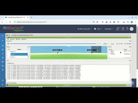
Nam Outputs

The Results of Some Elementary Analysis

             
In the following graphs, the firs one compare 4 algorithms (diffusion-rate, diffusion-prob, omnicast and flooding) and the second one compares 3 algorithms (without flooding) for clarity.

In the following graph high PDF signifies better Performance (in this graph, the pdf is greater than 100 because, in all these compared routing algorithms, the received packets may be always higher than that of sent packets because,  these algorithms will deliver same packet over different path.0

In the following graph low End-to-End Delay signifies better Performance

In the following graph  low number of  dropped Packets signifies better Performance

 

 

In the following graphs Minimum Routing Load signifies better Performance

 

In the following graph, High Remaining Battery power signifies better Performance

 

 

Conclusion:

Directed Diffusion is a method of data dissemination especially suitable in distributed sensing scenarios. It differs from IP method of communication. For IP “nodes are identified by their end-points, and inter-node communication is layered on an end-to-end delivery service provided within the network”. Directed diffusion, on the other hand is data-centric. Data generated by sensor nodes are identified by their attribute-value pair. Sinks or nodes that request data send out “interest”s into the network. Data generated by “source” nodes that match these interests, “flow” towards the sinks. Intermediate nodes are capable of caching and transforming data.

Using directed diffusion one can realize robust multi-path delivery, empirically adapt to a small subset of network paths, and achieve significant energy savings when intermediate nodes aggregate responses to queries.