Simulation of Hierarchical Sensor Network Topology in ns-2

An Example of Hierarchical Sensor Network

The following diagram shows a typical hierarchical sensor network topology. In this example, we will see a Tcl code that can be used to create a three-level hierarchical wireless sensor network.

The Code Fragment used in the creation of the 3 level Hierarchical Sensor Network.

# variables which control the number of Sensor nodes, fusion nodes & base station and how they're grouped
# (see topology creation code below)

set NumberOfBaseStations 1 ;# Always 1 in this Project
set SizeOfBaseStationNode 50 ;#

set NumberOfFusionSensorNodes 7 ;#
set SizeOfFusionSensorNode 40 ;#

set NumberOfNormalSensorNodesPerLevel 20 ;#
set SizeOfNormalSensorNode 30 ;#

set NumberofLayersAt0Level 1 ;#

set GapBetweenNormalSensorNodes 75 ;#
set GapBetweenFusionSensorNodes 150 ;#

set DistanceBetweenFusionSensorNodesAndBaseStationNode 250 ;#
set DistanceBetweenFusionSensorNodesAndNormalSensorNodes 75 ;#

set TotalNodes [expr $NumberOfBaseStations + $NumberOfFusionSensorNodes + $NumberOfNormalSensorNodesPerLevel* $NumberofLayersAt0Level]







set ns [new Simulator]


# set up topography object
set topo [new Topography]

$topo load_flatgrid $val(x) $val(y)

#
# Create God
#
create-god $TotalNodes 


# create the BS

 set n(0) [$ns node]
 $n(0) color "green"

 $n(0) set X_ [expr $val(x)/2]
 $n(0) set Y_ [expr $val(y)- 100 ]
 $n(0) set Z_ 0.0
 $ns initial_node_pos $n(0) $SizeOfBaseStationNode

# Create the Fusion Nodes 
for {set j 0} {$j < $NumberOfFusionSensorNodes} {incr j} {
 set i [ expr $j +1 ]
 set n($i) [$ns node]
 $n($i) color "blue"
 
 $n($i) set X_ [expr ($val(x)/2 - $NumberOfFusionSensorNodes/2 * $GapBetweenFusionSensorNodes) + ($GapBetweenFusionSensorNodes *$j) ]
 $n($i) set Y_ [expr $val(y)- 100 - $DistanceBetweenFusionSensorNodesAndBaseStationNode ]
 $n($i) set Z_ 0.0
 
 $ns initial_node_pos $n($i) $SizeOfFusionSensorNode 
}

# Create the Normal Nodes 
for {set k 0} {$k < $NumberofLayersAt0Level } {incr k} {

 for {set j 0} {$j < $NumberOfNormalSensorNodesPerLevel} {incr j} {
 
 set i [ expr $j + 1 + $NumberOfFusionSensorNodes + ($NumberOfNormalSensorNodesPerLevel * $k )]
 set n($i) [$ns node]
 $n($i) color "black"
 
 $n($i) set X_ [expr ($val(x)/2 - $NumberOfNormalSensorNodesPerLevel/2 * $GapBetweenNormalSensorNodes) + ($GapBetweenNormalSensorNodes *$j) ]
 $n($i) set Y_ [expr $val(y)- 100 - $DistanceBetweenFusionSensorNodesAndBaseStationNode - $DistanceBetweenFusionSensorNodesAndNormalSensorNodes - ($GapBetweenNormalSensorNodes * $k)]
 $n($i) set Z_ 0.0
 
 $ns initial_node_pos $n($i) $SizeOfNormalSensorNode
 }

}

If we use the above segment of code in our simulation, then we can create topologies shown below.

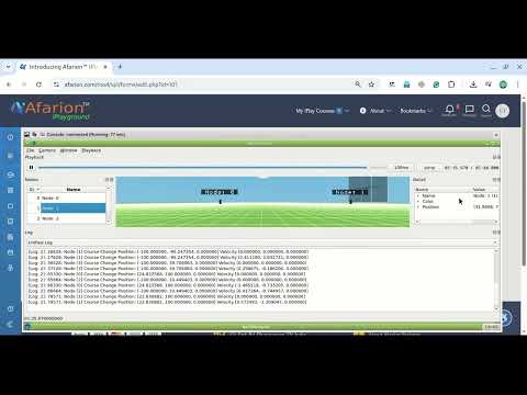
A Three-Level Hierarchical Sensor Network Sensor network Simulated in ns2 and visualized in Nam.

A Three-Level Hierarchical Sensor Network Sensor network with 6 layers of normal sensor nodes at the 0th Level.

A Three-Level Hierarchical Sensor Network Sensor network with randomly placed sensor nodes at the 0th Level.