Discuss Through WhatsApp
ns-3.38+ / AI & DRL
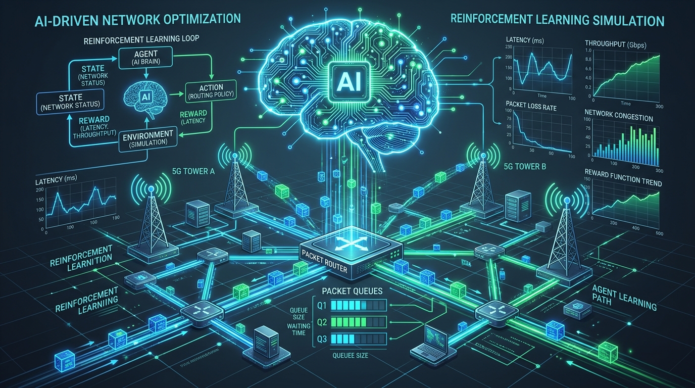
An exhaustive exploration of integrating modern Deep Reinforcement Learning (DRL) with the ns-3 discrete-event network simulator. This guide dissects high-performance IPC engines (ns3-ai), the Gymnasium environment abstraction, mathematical modeling of learning-based congestion control and 5G RAN resource allocation, and delivers an uncompromising engineering reality check on whether AI can truly replace classical networking heuristics.
1. The Paradigm Shift: From Handcrafted Heuristics to Autonomy
For more than four decades, computer networking has thrived on handcrafted heuristics. From Van Jacobson’s seminal additive-increase multiplicative-decrease (AIMD) algorithm in TCP Reno to the cubic curves of TCP Cubic, and from Bellman-Ford shortest-path routing to 3GPP Proportional Fair radio scheduling, protocols have been engineered using intuitive, closed-form control theory.
While these classical algorithms provide mathematical tractability, provable stability, and minimal computational overhead, they rely on a foundational assumption: the underlying operating environment conforms to idealized, stationary statistical models. However, modern communication networks have evolved into hyper-complex, non-stationary ecosystems:
- 5G/6G Heterogeneous Networks: Millimeter-wave (mmWave) and sub-THz channels undergo sudden, deep blockages spanning 20–30 dB within milliseconds, defying classical Poisson or Markovian fading approximations.
- Mega-Constellation LEO Satellites: Starlink-like networks experience continuously shifting Doppler shifts, high propagation delays, and ultra-dynamic inter-satellite link (ISL) topologies.
- Multi-Tenant Datacenter Fabrics: Incast traffic, microbursts, and partition-aggregate workloads drive packet buffers from zero to complete exhaustion within dozens of microseconds.
In response, the networking research community has increasingly turned toward Deep Reinforcement Learning (DRL). Unlike supervised learning, which requires massive labeled datasets of past packet traces, DRL learns optimal control policies by directly interacting with the network: observing states ($s_t$), taking discrete or continuous actions ($a_t$), and receiving scalar rewards ($r_t$) derived from throughput, latency, and packet loss.
2. Architectural Frameworks: Bridging ns-3 with Modern AI
ns-3 is a high-performance, discrete-event network simulator engineered in C++. Modern deep reinforcement learning frameworks (such as PyTorch, TensorFlow, and Stable-Baselines3), however, are overwhelmingly native to Python. Bridging these two distinct environments has historically been the primary bottleneck in learning-based networking research.
2.1 The Inter-Process Communication (IPC) Bottleneck
Early attempts at coupling ns-3 with AI algorithms relied on rudimentary IPC mechanisms:
- File I/O (CSV / JSON Traces): ns-3 dumped packet traces to disk, a Python script parsed them, updated the model, and wrote action files for ns-3 to ingest. This incurred massive disk I/O latency, limiting simulations to a few steps per second.
- Unix Domain Sockets & TCP/UDP Sockets: ns-3 acted as a socket client communicating with a Python server. While vastly faster than disk files, serialization overhead (e.g., Protobuf, JSON) and operating system kernel context switching created significant latency—often exceeding 2–5 milliseconds per interaction step. In simulations requiring millions of per-packet or per-slot control decisions, socket IPC reduced simulation throughput by orders of magnitude.
2.2 Deep Dive into ns3-ai: The Shared Memory Engine
The ns3-ai framework (developed by researchers at Huazhong University of Science and Technology) completely dismantled the IPC bottleneck by introducing a high-performance POSIX Shared Memory (shm) abstraction.
Rather than serializing packets over network sockets, ns3-ai maps a shared physical memory segment directly into the address spaces of both the C++ ns-3 simulation process and the Python AI process.
struct EnvFeature {
float throughput; // Current delivery rate (Mbps)
float rttGradient; // RTT_curr / RTT_min
float lossRate; // Fraction of packets dropped
float bytesInFlight; // Unacknowledged bytes
};
struct ActFeature {
float cwndMultiplier; // Multiplicative factor for Congestion Window
float pacingRateFactor; // Pacing rate adjustment factor
};
Key architectural properties of ns3-ai include:
- Zero-Copy Data Transfer: C++ pointers write state data directly into shared memory. On the Python side, NumPy arrays wrap the exact same raw memory buffer without copying data across process boundaries.
- Sub-Microsecond Synchronization: Process coordination is handled via atomic flags and POSIX condition variables/semaphores, dropping interaction latency down to under 1.5 microseconds per step—a 1000x improvement over network sockets.
- Non-Intrusive Integration: ns-3 code can be instrumented anywhere (in
TcpCongestionOps, MAC schedulers, or routing protocols) via concise C++ helper classes.
2.3 The Gymnasium Standard (gym.Env)
To enable seamless compatibility with modern RL algorithms (such as PPO, SAC, DDPG, and DQN), the network simulation must be formulated as a standard Gymnasium (formerly OpenAI Gym) environment conforming to the classical Markov Decision Process (MDP) API:
reset(seed=None, options=None): Initializes or re-seeds the ns-3 simulation topology, sets random traffic generators, and returns the initial observation $s_0$.step(action): Applies the AI’s action $a_t$ (e.g., updating a TCP congestion window or allocating subcarrier resource blocks), advances the ns-3 discrete-event clock by duration $Delta t$, and returns(observation, reward, terminated, truncated, info).observation_space: Defines the mathematical bounds and dimensionality of observations, typically usingspaces.Box(low=0.0, high=np.inf, shape=(N,), dtype=np.float32).action_space: Defines whether actions are continuous (e.g., pacing rate multiplier $in [0.5, 2.0]$) or discrete (e.g., selecting one of $K$ radio channels).
3. AI ↔ ns-3 Simulation Integration Architecture
The interaction between the discrete-event C++ simulator and the asynchronous Python deep learning engine is a closed feedback loop coordinated across three structural tiers:
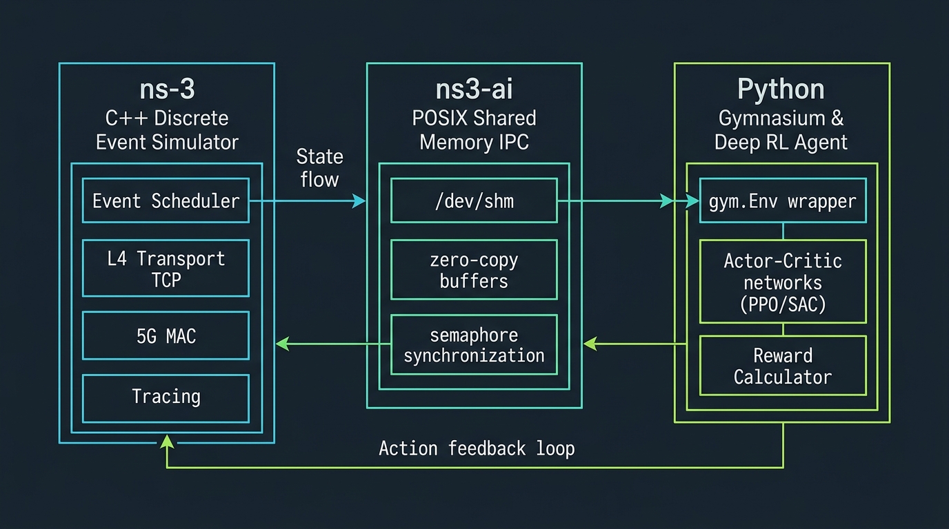
ns3-ai POSIX shared memory layer, and the Python Gymnasium deep reinforcement learning agent.
sequenceDiagram
    autonumber
    participant DRL as Python DRL Agent (PPO/SAC)
    participant Gym as Gymnasium Wrapper (gym.Env)
    participant Shm as ns3-ai Shared Memory (/dev/shm)
    participant ns3 as ns-3 Simulation Engine (C++)

    DRL->>Gym: env.reset()
    Gym->>Shm: Send reset control flag
    Shm->>ns3: Trigger topology setup & seed
    ns3->>Shm: Write initial features s_0
    Shm->>Gym: Map NumPy array s_0
    Gym->>DRL: Return initial observation s_0

    loop Every Interaction Step t
        DRL->>DRL: Evaluate Policy π(a_t | s_t)
        DRL->>Gym: env.step(action a_t)
        Gym->>Shm: Write action struct & signal semaphore
        Shm->>ns3: Unblock event loop; inject action a_t
        Note over ns3: Simulator runs for duration Δt
Packets forwarded, queues updated
        ns3->>Shm: Write new metrics (throughput, RTT, loss)
        Shm->>Gym: Signal step completion
        Gym->>Gym: Calculate scalar reward r_t
        Gym->>DRL: Return (s_{t+1}, r_t, terminated, truncated, info)
        DRL->>DRL: Store transition & optimize neural weights
    end
4. Case Study 1: RL-Powered Transport Layer Congestion Control
Congestion control represents one of the most prominent application domains for reinforcement learning in networking. Classic algorithms suffer from inherent design compromises:
- Loss-Based (Cubic, Reno): Require buffer queue fill-up until packet loss occurs, inducing severe bufferbloat and destructive queuing delay in high-speed networks.
- Model/Rate-Based (BBRv1, BBRv2, BBRv3): Explicitly estimate bottleneck bandwidth ($BtlBw$) and round-trip propagation time ($RTprop$). However, they frequently struggle with fairness when competing against aggressive loss-based flows and can suffer from bandwidth mis-estimation under high non-congestive loss.
- Performance-Oriented / Learning-Based (PCC Vivace, Aurora, Orca): Observe empirical transfer utility over micro-epochs and adjust transmission rates dynamically.
4.1 The Challenge: High-Bandwidth, High-Delay (BDP) Paths
In high Bandwidth-Delay Product (BDP) environments—such as 10 Gbps inter-datacenter links, trans-oceanic cables, or Low Earth Orbit (LEO) satellite constellations (e.g., 50 ms delay with 500 Mbps capacity):
- Additive-increase heuristics take tens or hundreds of RTTs to utilize spare link capacity after a route switch.
- Transient wireless channel drops (e.g., rain fade or beam misalignment) are mistaken for network congestion, causing traditional TCP to slash its congestion window by 50% unnecessarily.
4.2 Mathematical MDP Formulation for Congestion Control
We formulate the congestion control challenge as a continuous-control Markov Decision Process:
State / Observation Space ($s_t in mathbb{R}^6$)
Over an observation epoch $[t, t + Delta t]$ (typically 1 RTT interval):
1. Normalized Delivery Rate: $hat{x}_t = frac{text{AckedBytes}_t}{Delta t cdot C_{text{est}}}$
2. RTT Gradient: $g_t = frac{text{RTT}_{text{curr}}}{text{RTT}_{text{min}}}$ (signaling queue inflation)
3. RTT Variance: $sigma_{text{RTT}} = frac{text{Var}(text{RTT})}{(text{RTT}_{text{min}})^2}$
4. Packet Loss Ratio: $L_t = frac{text{PacketsLost}_t}{text{PacketsSent}_t}$
5. Inflight-to-BDP Ratio: $rho_t = frac{text{BytesInFlight}_t}{text{BDP}_{text{est}}}$
6. ECN Ratio: $E_t = frac{text{ECN_Marked_Packets}_t}{text{Total_Acks}_t}$
Action Space ($a_t in mathbb{R}^2$)
Continuous pacing rate and window adjustments:
1. Pacing Rate Factor ($alpha_t in [0.5, 2.0]$): Multiplies current pacing rate: $text{Rate}_{t+1} = alpha_t cdot text{Rate}_t$
2. Congestion Window Multiplier ($beta_t in [0.5, 1.5]$): $text{Cwnd}_{t+1} = beta_t cdot text{Cwnd}_t$
Multi-Objective Reward Function ($r_t$)
Balancing high delivery rate against queueing delay (Kleinrock’s power metric with loss penalty):
Where $lambda_1, lambda_2, lambda_3$ are penalty weights discouraging bufferbloat, packet drops, and early congestion markings respectively.
4.3 C++ ns-3 Implementation Hook (TcpRlCc)
In ns-3, we implement a custom congestion control algorithm deriving from TcpCongestionOps:
#include “ns3/tcp-congestion-ops.h”
#include “ns3/ns3-ai-module.h”
class TcpRlCc : public TcpCongestionOps {
public:
static TypeId GetTypeId(void) {
static TypeId tid = TypeId(“ns3::TcpRlCc”)
.SetParent
.AddConstructor
return tid;
}
virtual void PktsAcked(Ptr
m_bytesAckedEpoch += segmentsAcked * tcb->m_segmentSize;
m_minRtt = std::min(m_minRtt, rtt);
m_lastRtt = rtt;
// When epoch expires (e.g. 1 RTT interval)
if (Simulator::Now() – m_epochStart >= m_lastRtt) {
SendFeaturesAndApplyAction(tcb);
m_epochStart = Simulator::Now();
m_bytesAckedEpoch = 0;
}
}
private:
void SendFeaturesAndApplyAction(Ptr
// 1. Write state vector to ns3-ai shared memory pool
auto feat = s_shm->GetFeaturePool();
feat->deliveryRate = (m_bytesAckedEpoch * 8.0) / (m_lastRtt.GetSeconds() * 1e6);
feat->rttGradient = m_lastRtt.GetSeconds() / m_minRtt.GetSeconds();
feat->lossRate = (double)m_lostSegmentsEpoch / std::max(1u, m_sentSegmentsEpoch);
feat->bytesInFlight = tcb->m_bytesInFlight.Get();
s_shm->NotifyFeatureReady();
// 2. Wait for Python DRL agent to write action to shared memory
s_shm->WaitForAction();
auto act = s_shm->GetActionPool();
// 3. Apply continuous actions to TCP state machine
uint32_t newCwnd = tcb->m_cWnd * act->cwndMultiplier;
tcb->m_cWnd = std::max(newCwnd, 2 * tcb->m_segmentSize);
tcb->SetPacingRate(tcb->GetPacingRate() * act->pacingRateFactor);
}
};
4.4 Python Gymnasium Agent Implementation
import gymnasium as gym
from gymnasium import spaces
import numpy as np
from py_ns3_ai import Ns3ShmBridge
from stable_baselines3 import PPO
class Ns3TcpCongestionEnv(gym.Env):
def __init__(self):
super().__init__()
# State: [deliveryRate, rttGradient, lossRate, bytesInFlight]
self.observation_space = spaces.Box(low=0.0, high=np.inf, shape=(4,), dtype=np.float32)
# Action: [cwndMultiplier in [0.5, 1.5], pacingFactor in [0.5, 2.0]]
self.action_space = spaces.Box(low=np.array([0.5, 0.5]), high=np.array([1.5, 2.0]), dtype=np.float32)
self.shm = Ns3ShmBridge(shared_mem_key=“ns3_tcp_pool”)
def step(self, action):
# 1. Write action into shared memory
self.shm.write_action({“cwndMultiplier”: action[0], “pacingRateFactor”: action[1]})
# 2. Synchronize and read updated observation from ns-3
obs_dict = self.shm.read_features()
obs = np.array([obs_dict[‘deliveryRate’], obs_dict[‘rttGradient’],
obs_dict[‘lossRate’], obs_dict[‘bytesInFlight’]], dtype=np.float32)
# 3. Calculate multi-objective utility reward
tput = max(obs_dict[‘deliveryRate’], 1e-3)
rtt_ratio = max(obs_dict[‘rttGradient’], 1.0)
reward = np.log(tput) – 1.5 * np.log(rtt_ratio) – 10.0 * obs_dict[‘lossRate’]
terminated = obs_dict.get(‘sim_done’, False)
return obs, float(reward), terminated, False, {}
# Train PPO Agent directly against ns-3
env = Ns3TcpCongestionEnv()
model = PPO(“MlpPolicy”, env, verbose=1, learning_rate=3e-4, gamma=0.99)
model.learn(total_timesteps=200_000)
5. Case Study 2: Intelligent Radio Access Network (RAN) Resource Allocation
Beyond the transport layer, Reinforcement Learning is extensively researched across the cellular Radio Access Network (RAN), where complex multi-variable constraints outstrip classical heuristics.
5.1 DRL-Based Spectrum Sensing in Cognitive Radio
In cognitive radio networks, secondary users (SUs) must opportunistically transmit across licensed channels without interfering with Primary Users (PUs). Classical energy detection requires constant spectral scanning, which drains battery power and consumes valuable transmission time.
By framing the multi-channel occupancy as a Partially Observable Markov Decision Process (POMDP), a Deep Q-Network (DQN) observes historical PU arrival statistics and predicts which channel has the highest probability of remaining idle in the next slot. In ns-3, this is simulated using the SpectrumChannel model, where the DQN agent selectively samples only 1 out of $M$ channels, achieving over 90% transmission opportunity capture while slashing radio sensing energy by 75%.
5.2 Dynamic Channel Allocation & 5G-NR RAN Slicing
5G networks multiplex radically diverse traffic profiles over a shared physical channel:
- Enhanced Mobile Broadband (eMBB): Bandwidth-hungry, high throughput, delay-tolerant.
- Ultra-Reliable Low-Latency Communication (URLLC): Microsecond deadlines ($≤ 1text{ ms}$), 99.999% packet success rate, bursty arrivals.
- Massive Machine-Type Communications (mMTC): Dense sensor telemetry, low data rate.
Classical MAC schedulers (Round Robin, Proportional Fair) allocate Physical Resource Blocks (PRBs) statically or greedily based on instantaneous channel quality. However, an unexpected URLLC burst requires immediate puncturing or preemption of ongoing eMBB transmissions.
A DRL actor embedded in the gNB MAC layer dynamically splits the Bandwidth Part (BWP) into flexible slice quotas every 10 ms. The reward function enforces a non-linear SLA barrier penalty:
The exponential penalty prevents even a single URLLC packet from violating its strict latency deadline, training the agent to maintain an adaptive headroom buffer for unexpected bursts without starving eMBB flows.
5.3 Proactive Handover Management in Mobile Scenarios
The standard 3GPP handover mechanism relies on Event A3: when a neighbor cell’s Reference Signal Received Power (RSRP) exceeds the serving cell’s RSRP by a fixed hysteresis margin ($Hys$) for a specified Time-to-Trigger ($TTT$).
In vehicular (V2X) and high-speed rail scenarios (120–300 km/h), this static rule inevitably fails:
- Too short TTT: Causes severe handover ping-pong between base stations, generating massive signaling storm overhead.
- Too long TTT: The vehicle outruns the serving cell coverage before the handover completes, resulting in abrupt Radio Link Failure (RLF).
Using ns-3 mobility models (such as ConstantVelocityMobilityModel and Ns2MobilityHelper), an actor-critic DRL agent takes as input a rolling window of past RSRP, RSRQ, Doppler velocity, and target cell load. Rather than reacting to historical thresholds, the policy anticipates upcoming shadow fading dips and executes proactive handovers, eliminating both ping-pong oscillation and link dropouts.
6. Critical Engineering Discussion: The Reality Check
Having explored the theoretical elegance and simulation success of DRL in ns-3, we must confront the central questions that every rigorous network researcher and systems engineer must answer:
“Can AI-based algorithms really compete with simple classical algorithms in the real world? Is AI genuinely necessary for simple networking tasks?”
While academic literature frequently showcases impressive graphs showing DRL beating TCP Cubic or Round-Robin by 15–20% on specific benchmark topologies, deploying these models in production uncovers formidable architectural barriers.
6.1 The Nanosecond Line-Rate Reality
The most brutal reality of computer networking is line-rate physics. Modern switches, routers, and Network Interface Cards (NICs) process packets at 100 Gbps, 400 Gbps, and 800 Gbps:
- At 100 Gbps, a standard 64-byte minimum-size Ethernet frame arrives every 5.12 nanoseconds.
- At 400 Gbps, the packet inter-arrival window shrinks to 1.28 nanoseconds.
In contrast, executing even a tiny 2-layer Multi-Layer Perceptron (MLP) using a dedicated hardware accelerator (NPU or TensorRT-quantized INT8 engine) consumes 5 to 50 microseconds. Calling a neural network inference for every packet arrival is three to four orders of magnitude too slow.
Classical algorithms (like TCP Cubic, BBR, CoDel, or WRED) calculate their state transitions using simple arithmetic: a few additions, bit shifts, and comparisons that execute in sub-nanosecond CPU clock cycles directly inside the kernel network stack or in P4-programmable ASIC pipelines.
6.2 The Generalization & Sim-to-Real Chasm
Reinforcement learning policies trained in simulated ns-3 environments suffer from severe out-of-distribution (OOD) brittleness:
- Synthetic Overfitting: A DRL congestion control policy trained on a dumbbell topology with static bottleneck bandwidth and Pareto cross-traffic will learn subtle statistical artifacts unique to that exact synthetic distribution.
- Catastrophic Collapse in the Wild: When deployed against unexpected real-world conditions—such as cellular bufferbloat, unannounced ACK compression on Wi-Fi links, or adversarial packet bursts—the neural network enters unmapped regions of its state space. Unlike classical algorithms that gracefully degrade back to conservative AIMD, DRL policies can experience catastrophic policy collapse, driving packet loss to 100% or inducing total flow starvation.
6.3 Provable Stability vs Black-Box Unpredictability
Network infrastructure is critical mission-oriented systems software. Internet service providers (ISPs) and enterprise operators prioritize predictability and bounded worst-case performance above all else:
- Classical Heuristics: Can be rigorously modeled using Lyapunov control theory, fluid-flow differential equations, and Markov chains. They offer mathematical proofs of convergence, boundedness, and max-min fairness. When an anomaly occurs, an engineer can trace the exact
if/elsebranch that triggered it. - Deep Neural Networks: Are opaque, non-linear black-box function approximators containing millions of floating-point weights. They cannot provide hard guarantees against route oscillations, routing loops, or catastrophic queue starvation. In a production outage, explaining why a neural network selected an erroneous action vector is virtually impossible.
6.4 Engineering Cost & Energy Footprint
Deploying a classical heuristic requires 15 to 50 lines of robust, static C++ code that can run on an inexpensive micro-controller or embedded router CPU for years without maintenance. Training and maintaining a DRL policy requires:
- Expensive GPU clusters running millions of simulation episodes.
- Continuous monitoring for concept drift and non-stationary environment changes.
- Continuous retraining pipelines to prevent stale policy degradation.
6.5 The Architectural Comparison Matrix
6.6 The Verdict: Where AI Belongs vs Where Heuristics Rule
To conclude honestly: AI is NOT needed for simple networking tasks. For point-to-point packet forwarding, FIFO/RED queue management, or standard intra-datacenter congestion control on stable fiber links, applying deep reinforcement learning is an over-engineered anti-pattern that introduces unnecessary complexity, latency, and instability.
However, AI shines brilliantly when applied to the right timescale and abstraction layer:
❌ Where AI Fails (Microsecond Fast-Path)
- Per-packet forwarding and lookup tables.
- Per-ACK window adjustments on sub-millisecond LANs.
- Basic static or shortest-path routing.
- Active queue management (AQM) on line-rate switches.
✅ Where AI Excels (Macroscopic Slow-Path)
- 5G/6G Network Slicing & PRB quota optimization (10–100 ms).
- Predictive multi-cell Handover & Beam steering in vehicular V2X.
- End-to-end Traffic Matrix engineering & WAN flow rerouting.
- Energy-saving massive MIMO antenna sleep scheduling.
The future of production networking is not an outright replacement of classical algorithms, but a hybrid two-tier architecture (as demonstrated by systems like Orca). In this model:
1. Classical heuristics run the deterministic fast-path (enforcing safety invariants, guaranteed minimum throughput, and immediate line-rate backoff).
2. A DRL agent runs in the background slow-path (at 50–200 ms intervals), observing macro-trends and tuning the operating parameters of the classical controller.
7. Conclusion & Research Roadmap
The integration of ns-3 with ns3-ai and Gymnasium has democratized cutting-edge AI research in telecommunications. By leveraging POSIX shared memory, researchers can bypass historical serialization bottlenecks and evaluate deep reinforcement learning policies across realistic 5G/6G, satellite, and transport layer topologies with sub-microsecond IPC latency.
Yet, true engineering progress demands intellectual humility. As you explore learning-based networking in ns-3, remember that the goal is not to force a neural network onto every packet header, but to identify the multi-dimensional, non-stationary optimization problems where heuristics genuinely falter—and to wrap every AI policy in a deterministic, safety-proven classical guardrail.
Written by Charles Pandian
Network simulation researcher and systems architect specializing in ns-2, ns-3, 5G-NR modeling, and high-performance cross-layer protocol engineering. Regular contributor to ProjectGuideline.com academic tutorials and simulation architectures.
 Take Me to Afarion ns-3 iPlayground